这篇文章是PointNet的续篇，网上也有很多说明博客，这里记录我觉得比较重要的Method部分
PS：这篇文章的一些代码注释感谢沈同学的一些帮助

Method

对于PointNet的介绍

PaperRead：PointNet：Deep Learning on Point Sets for 3D Classification and Segmentation

层次化点集特征学习

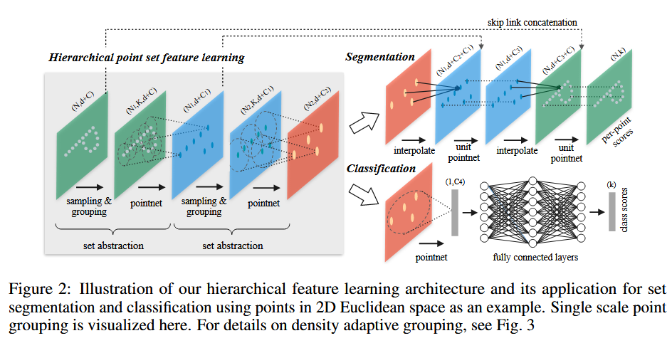
采样层

• FPS采样：就是第一次采样随机，之后第二次的点的选取，先要计算和第一个点的距离，然后我们有个distance矩阵进行更新，如果有更近的距离就更新矩阵，再全局搜索距离最短的点
  • 这里我刚开始有个误区，刚开始理解成了：随机选择点1，选择与点1距离最远的点2，选择与点2距离最远的点3，以此类推
  • 这种思路是错误的，因为我们的distance信息是基于前面几轮的，所以正确规则是随机选择点1，选择与点1距离最远的点2， 接下来，要选择点3。规则是：对于点云中每一个尚未被选择的点，我们计算它到点1的距离和到点2的距离，然后取这两者中的较小值。我们的目标是找到那个“较小值”最大的点，这个点就是点3。在选择点4时，也是同理：对于每一个尚未被选择的点，我们计算它到{点1, 点2, 点3}这个集合的“最短距离”，然后选择那个“最短距离”最大的点作为点4。
  • 这样我们就能用几个点尽可能分布整个点云

# 对点云进行采样，个数为npoint，选取规则为迭代最远采样（FPS）
def farthest_point_sample(xyz, npoint):
    # xyz为数据，npoint为采样点数
    """
    Input:
        xyz: pointcloud data, [B, N, 3]
        npoint: number of samples
    Return:
        centroids: sampled pointcloud index, [B, npoint]
    """
    device = xyz.device
    B, N, C = xyz.shape
    # 初始化采样点集，大小为(B,npoint)
    centroids = torch.zeros(B, npoint, dtype=torch.long).to(device)
    # 初始化距离矩阵，大小为(B,N)，数值均为1x10的十次方 [B, N]
    distance = torch.ones(B, N).to(device) * 1e10
    # 生成一个长为B的数组，里面数值范围为0~N，即在每个batch中随机抽取一个点进入点集，代表着点集的索引
    farthest = torch.randint(0, N, (B,), dtype=torch.long).to(device)
    # 生成一个长为B的数组，[0,1,2,...,B-1]
    batch_indices = torch.arange(B, dtype=torch.long).to(device)
    for i in range(npoint):
        #  更新第i个最远点，第一个最远点（i=1）为随机抽取
        centroids[:, i] = farthest
        #  将选取的点的xyz存入centroid
        centroid = xyz[batch_indices, farthest, :].view(B, 1, 3)
        #  计算点集中的所有点到这个最远点的欧式距离[B, N]
        dist = torch.sum((xyz - centroid) ** 2, -1) 
        #  更新distances，记录样本中每个点距离所有已出现的采样点的最小距离
        mask = dist < distance  #  生成一个值为0和1的掩码 [B, N]
        # 更短的新距离，这里包括i-1轮
        distance[mask] = dist[mask] # “布尔索引”或“掩码索引”
        # 从更新后的distances矩阵中找出距离最远的点，作为最远点用于下一轮迭代
        # torch.max(distance, -1)取出每一行的最大值构成列向量，等价于torch.max(x,2)
        # torch.max(distance, -1)[1]是取列向量的索引，若torch.max(distance, -1)[0]则是取列向量
        # 在distance的每一行中找到最大值的索引，这个索引就是下一个最远点。它的形状仍然是 [B]。
        farthest = torch.max(distance, -1)[1]
    # 返回采样所选取的点集，大小为(B,npoint)
    return centroids

分组层

• 球形查询会找到查询点半径范围内的所有点（在执行过程中设置了 K 的上限）
• 这里如果我们每个中心K半径内的点数满足数量那就很好说了，如果小于半径点数我们该怎么办呢？
• 我们的做法是 group_idx 中所有的多余的 N 都被替换成了该区域找到的第一个点的索引，保证输出的索引都是有效的。
• 这样我们的输出就是个固定的表示

# 对应于Grouping layer, 这一层使用Ball query方法生成N'个局部区域，根据论文中的意思，这里有两个变量 ，一个是每个区域中点的数量K，
# 另一个是球的半径。这里半径应该是占主导的，会在某个半径的球内找点，上限是K
def query_ball_point(radius, nsample, xyz, new_xyz):
    # 输入中radius为球形领域的半径，nsample为每个领域中要采样的点，new_xyz为S个球形领域的中心（由最远点采样在前面得出），
    # xyz为所有的点云；输出为每个样本的每个球形领域的nsample个采样点集的索引[B,S,nsample]。
    """
    Input:
        radius: local region radius
        nsample: max sample number in local region
        xyz: all points, [B, N, 3]
        new_xyz: query points, [B, S, 3]
    Return:
        group_idx: grouped points index, [B, S, nsample]
    """
    device = xyz.device
    # B为batch_size，N为点云数量，C为通道数量，这里为3(x,y,z)
    B, N, C = xyz.shape
    # S为迭代最远采样选取的中心点的个数
    _, S, _ = new_xyz.shape
    # torch.arange(N)可以生成tensor([0,1,...,N-1])
    # 最后group_idx的大小为(B,S,N),最后一个维度均为tensor([0,1,...,N-1])
    group_idx = torch.arange(N, dtype=torch.long).to(device).view(1, 1, N).repeat([B, S, 1])
    # 计算中心点位与所有点位的距离的平方，sqrdists大小为(B,S,N),存储的是距离矩阵
    sqrdists = square_distance(new_xyz, xyz)
    # radius ** 2代表半径的平方，即：令group_idx中所有距离大于半径的点设为N
    group_idx[sqrdists > radius ** 2] = N
    # 对group_idx进行升序排列，输出为(B,S,nsample)，即选取前nsample个点
    group_idx = group_idx.sort(dim=-1)[0][:, :, :nsample]
    # 处理“空位”的“补位”技巧
    # 输出为(B,S,nsample),最后一个维度的值均为第一个距离中心点小于半径的点的索引，
    group_first = group_idx[:, :, 0].view(B, S, 1).repeat([1, 1, nsample])
    # mask为掩码，大小为(B,S,N)，值为1代表该点距离大于半径，值为0代表该点的距离小于等于半径
    mask = group_idx == N
    group_idx[mask] = group_first[mask]
    # 到此返回的分组既满足了半径又满足了个数
    return group_idx

• 这里是把两个部分结合起来成为图片过程中的一层，下面这段代码也包括局部区域内的点的坐标首先被转换为相对于中心点的局部坐标系的过程

# 将整个点云分散成局部的group
def sample_and_group(npoint, radius, nsample, xyz, points, returnfps=False):
    """
    Input:
        npoint:FPS采样点的数量，即分组的数量
        radius:球形区域所定义的半径
        nsample:球形区域所能包围的最大的点数量
        xyz: input points position data, [B, N, 3]，原始点云数据
        points: input points data, [B, N, D]，除了xyz坐标外，其余特征维度，例如：颜色，热力
    Return:
        new_xyz: sampled points position data, [B, npoint, nsample, 3]
        new_points: sampled points data, [B, npoint, nsample, 3+D]
    """
    # B为batch_size,N为点的个数,C为3(xyz)
    B, N, C = xyz.shape
    # S为采样点的数量
    S = npoint
    # 用farthest_point_sample函数实现最远点采样FPS得到采样点的索引
    fps_idx = farthest_point_sample(xyz, npoint) # [B, npoint]
    # 通过index_points将这些点的从原始点中挑出来，作为new_xyz，真实坐标
    new_xyz = index_points(xyz, fps_idx) # [B, npoint, C]
    # 利用query_ball_point和index_points将原始点云通过new_xyz 作为中心分为npoint个球形区域其中每个区域有nsample个采样点
    idx = query_ball_point(radius, nsample, xyz, new_xyz)
    grouped_xyz = index_points(xyz, idx) # [B, npoint, nsample, C]
    # 每个区域的点减去区域的中心值,进行局部分组的中心化
    grouped_xyz_norm = grouped_xyz - new_xyz.view(B, S, 1, C)

    # 如果每个点上面有新的特征的维度，则用新的特征与旧的特征拼接
    if points is not None:
        # 通过index_points将分组的点从points(B,N,D)中挑出来，作为grouped_points，即：将FPS筛选出来的点的其余特征维度提取出来
        grouped_points = index_points(points, idx)
        # 将中心化后的局部点的xyz坐标与其余特征拼接起来
        new_points = torch.cat([grouped_xyz_norm, grouped_points], dim=-1) # [B, npoint, nsample, C+D]
    # 如果每个点上面没有新的特征的维度，则直接返回中心化后的xyz特征
    else:
        new_points = grouped_xyz_norm

    # returnfps为False,则返回FPS挑选出来的中心点的xyz(new_xyz),中心化分组完成的点云数据(new_points)
    # returnfps为True,则返回上述两个外，返回未中心化分组后的点云数据(grouped_xyz),FPS挑选出来的中心点的索引(fps_idx)
    if returnfps:
        return new_xyz, new_points, grouped_xyz, fps_idx
    else:
        return new_xyz, new_points

Pointnet层

• PyTorch的 Conv2d 期望输入格式为 [批次, 通道数, 高, 宽]
• 里面的结构跟PointNet差不多，一个conv，一个BN，一个Relu
• 之后maxpooling将 K 个邻居点的信息聚合成了一个单独的、最能代表该区域特征的向量。new_points 的形状从 [B, D', K, S] 变成了 [B, D', S]

# new_xyz: sampled points position data, [B, npoint, C]
        # new_points: sampled points data, [B, npoint, nsample, C+D]
        new_points = new_points.permute(0, 3, 2, 1) # [B, C+D, nsample,npoint]
        # 利用1x1的2d的卷积相当于把每个group当成一个通道，共npoint个通道，
        # 对[3+D, nsample]的维度上做逐像素的卷积，结果相当于对单个C+D维度做1d的卷积
        for i, conv in enumerate(self.mlp_convs):
            bn = self.mlp_bns[i]
            new_points =  F.relu(bn(conv(new_points)))

class PointNetSetAbstraction(nn.Module):
    def __init__(self, npoint, radius, nsample, in_channel, mlp, group_all):
        super(PointNetSetAbstraction, self).__init__()
        self.npoint = npoint
        self.radius = radius
        self.nsample = nsample
        # nn.ModuleList()用法，例如：self.layers = nn.ModuleList([
        #             nn.Linear(64, 128),
        #             nn.Linear(128, 1024)
        #         ])
        self.mlp_convs = nn.ModuleList()
        self.mlp_bns = nn.ModuleList()
        last_channel = in_channel
        for out_channel in mlp:
            self.mlp_convs.append(nn.Conv2d(last_channel, out_channel, 1))
            self.mlp_bns.append(nn.BatchNorm2d(out_channel))
            last_channel = out_channel
        self.group_all = group_all

    def forward(self, xyz, points):
        """
        N是输入点的数量，C是坐标维度(C=3)，D是特征维度（除坐标维度以外的其他特征维度)
        S是输出点的数量，C是坐标维度，D'是新的特征维度
        Input:
            xyz: input points position data, [B, C, N]
            points: input points data, [B, D, N]
        Return:
            new_xyz: sampled points position data, [B, C, S]
            new_points_concat: sample points feature data, [B, D', S]
        """
        xyz = xyz.permute(0, 2, 1)
        if points is not None:
            points = points.permute(0, 2, 1)

        # group_all为True时调用sample_and_group_all，将整个点云化为一组
        # group_all为False时调用sample_and_group，将整个点云分为多个局部
        if self.group_all:
            new_xyz, new_points = sample_and_group_all(xyz, points)
        else:
            new_xyz, new_points = sample_and_group(self.npoint, self.radius, self.nsample, xyz, points)

    
        # new_xyz: sampled points position data, [B, npoint, C]
        # new_points: sampled points data, [B, npoint, nsample, C+D]
        new_points = new_points.permute(0, 3, 2, 1) # [B, C+D, nsample,npoint]
        # 利用1x1的2d的卷积相当于把每个group当成一个通道，共npoint个通道，
        # 对[3+D, nsample]的维度上做逐像素的卷积，结果相当于对单个C+D维度做1d的卷积
        for i, conv in enumerate(self.mlp_convs):
            bn = self.mlp_bns[i]
            new_points =  F.relu(bn(conv(new_points)))

        # 对每个group做一个max pooling得到局部的全局特征,得到的new_points:[B,3+D,npoint]
        new_points = torch.max(new_points, 2)[0]
        new_xyz = new_xyz.permute(0, 2, 1)# [B, D', S]
        # 返回FPS选取的中心点的xyz数据(new_xyz),单一尺度提取的局部特征(new_points)，
        return new_xyz, new_points

非均匀采样密度下的稳健特征学习

• 由于部分点云区域的密度不同，为实现这一目标，提出了密度自适应 PointNet 层，该层能够在输入采样密度变化时，学习如何结合来自不同尺度的特征。所以将含有密度自适应 PointNet 层的分层网络称为 PointNet++
• 又分成两种类别多尺度分组（MSG），多分辨率分组（MRG）
  

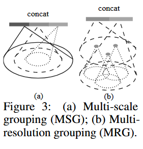
多尺度分组（MSG）

• 它的核心思想是，为了更鲁棒地学习特征，我们不应该只看一个固定大小的邻域，而应该同时观察好几个不同大小（不同半径）的邻域，然后把从这些不同尺度邻域中学到的特征组合起来。
• 这对于处理密度不均匀的点云尤其有效：在密度稀疏的区域，大的邻域能包含更多点，提供更稳定的上下文信息；在密度稠密的区域，小的邻域能捕捉到更精细的几何细节。
• 这里还是很好理解的：我是这么总结，先分不同的密度，在找不同数量对应的点，每个密度都会有一种MLP对应，最后并行后进行一个合并的操作
• 这里该博客的思考很有意思：pointnet-pp-Interpretion

# 捕获多尺度模式的方法是应用不同尺度的分组层，然后根据点来提取每个尺度的特征。将不同尺度的特征串联起来，形成多尺度特征。使用 Multi-Scale Grouping（MSG）方法的SA层
# 大部分的形式都与普通的SA层相似，但是这里radius_list输入的是一个list例如[0.1,0.2,0.4]，对于不同的半径做ball query，最终将不同半径下的点点云特征保存在new_points_list中，再最后拼接到一起
class PointNetSetAbstractionMsg(nn.Module):
    def __init__(self, npoint, radius_list, nsample_list, in_channel, mlp_list):
        super(PointNetSetAbstractionMsg, self).__init__()
        self.npoint = npoint
        self.radius_list = radius_list
        self.nsample_list = nsample_list
        self.conv_blocks = nn.ModuleList()
        self.bn_blocks = nn.ModuleList()
        for i in range(len(mlp_list)):
            convs = nn.ModuleList()
            bns = nn.ModuleList()
            last_channel = in_channel + 3
            for out_channel in mlp_list[i]:
                convs.append(nn.Conv2d(last_channel, out_channel, 1))
                bns.append(nn.BatchNorm2d(out_channel))
                last_channel = out_channel
            self.conv_blocks.append(convs)
            self.bn_blocks.append(bns)

    def forward(self, xyz, points):
        """
        Input:
            xyz: input points position data, [B, C, N]
            points: input points data, [B, D, N]
        Return:
            new_xyz: sampled points position data, [B, C, S]
            new_points_concat: sample points feature data, [B, D', S]
        """
        xyz = xyz.permute(0, 2, 1)
        if points is not None:
            points = points.permute(0, 2, 1)

        B, N, C = xyz.shape
        S = self.npoint
        # FPS选取中心点并且提取出数据
        new_xyz = index_points(xyz, farthest_point_sample(xyz, S))
        new_points_list = []
        # 根据radius_list和nsample_list中不同的半径和每个分组最多有的点数分别进行分组
        for i, radius in enumerate(self.radius_list):
            K = self.nsample_list[i]
            # 进行分组并提取数据
            group_idx = query_ball_point(radius, K, xyz, new_xyz)
            grouped_xyz = index_points(xyz, group_idx)
            # 对每个分组进行中心化
            grouped_xyz -= new_xyz.view(B, S, 1, C)
            # 如果每个点上面有新的特征的维度，则用新的特征与旧的特征拼接
            if points is not None:
                grouped_points = index_points(points, group_idx)
                grouped_points = torch.cat([grouped_points, grouped_xyz], dim=-1)
            # 如果每个点上面没有新的特征的维度，则直接返回中心化后的xyz特征
            else:
                grouped_points = grouped_xyz

            grouped_points = grouped_points.permute(0, 3, 2, 1)  # [B, D, K, S]
            # 进行mlp
            for j in range(len(self.conv_blocks[i])):
                conv = self.conv_blocks[i][j]
                bn = self.bn_blocks[i][j]
                grouped_points =  F.relu(bn(conv(grouped_points)))
            new_points = torch.max(grouped_points, 2)[0]  # [B, D', S]
            # 将局部特征加入到new_points_list
            new_points_list.append(new_points)

        # 输出为(B,S,D'),其中S为分组数量(FPS中心个数),D'为对3+D维进行mlp后的新维度
        new_xyz = new_xyz.permute(0, 2, 1)
        # 将不同半径和个数进行分组并对每个分组进行特征提取后的局部特征进行拼接
        new_points_concat = torch.cat(new_points_list, dim=1)
        # 返回FPS选取的中心点的xyz数据(new_xyz),不同尺度提取的局部特征拼接(new_points_concat)
        return new_xyz, new_points_concat

多分辨率分组（MRG）

• 这里没有官方代码的公布，这里我也没太理解（这个权重的设定问题，如何确定两个权重的值应该具体是什么样呢？阈值是什么样的呢？），这个问题有答案的uu可以在评论区留言
• 某一层级 的区域特征由两个向量拼接而成。第一个向量（图中左侧）是通过在下一层级 的子区域上使用集合抽象层对特征进行总结得到的；第二个向量（图中右侧）是通过直接处理局部区域中的所有原始点，使用单一的PointNet得到的特征。
• 当局部区域的点密度较低时，第一个向量可能会比第二个向量更不可靠，因为用于计算第一个向量的子区域包含的点更加稀疏，受采样不足的影响更大。在这种情况下，第二个向量的权重应更高。另一方面，当局部区域的点密度较高时，第一个向量由于能够通过递归的方式在较低层级中进行更高分辨率的观察，因此可以提供更细节的信息。
• 与MSG相比，该方法在计算上更高效，因为我们避免了在最低层级的大规模邻域中提取特征。

用于集合分割的点特征传播

• 如果把每层生成点特征都拼接回去，这可能会导致计算量太大的问题，这里作者不再使用简单的拼接，而是采用了插值+拼接的方式。用一句话概括，就是把全局特征按照距离权重散播到下一层的各点；下一层各点又按照距离权重散播到再下一层，直到转播到最后一层，即原始点。
• 每次传播，接收端的点都会将自身特征和接收的特征进行融合。这一层简称为FP层。
• 
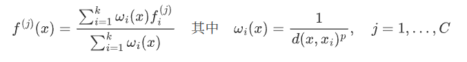
• 在多种插值方法中，我们使用基于k近邻的逆距离加权平均（如公式所示，默认情况下我们使用2，3）。点上插值得到的特征随后与集合抽象层的跳跃连接点特征拼接起来。然后，拼接后的特征通过一个“单位PointNet”处理，类似于CNN中的逐点卷积。接着应用若干共享的全连接层和ReLU层来更新每个点的特征向量。这个过程重复进行，直到我们将特征传播到原始点集。（原文的解释，我个人觉得有点难理解）
• 这里我那gemini给解释的例子说一下（个人觉得还挺好理解的）：
• 初始状态：
  • xyz1, points1 (密集点云): 这是我们想要预测的原始椅子上的 N=1024 个点。points1 可能只包含一些简单的低级特征，比如每个点周围的曲率，我们假设它是1维的。
  • xyz2, points2 (稀疏点云): 这是网络从深层学到的、包含高级语义的 S=2 个“精华点”。
  • 精华点 S1: 代表了“坐垫”这个概念。它的特征 points2[0] 是 [0.9, 0.1] (代表90%可能是坐垫, 10%可能是椅腿)。
  • 精华点 S2: 代表了“椅腿”这个概念。它的特征 points2[1] 是 [0.2, 0.8] (代表20%可能是坐垫, 80%可能是椅腿)。
• 现在，我们从 1024 个密集点中，随机挑一个点 P 来看看它经历了什么。假设点 P 物理上就位于椅子的坐垫上。
• 第一步：特征插值 (Interpolation)
  • 我们要为点 P 计算出一个高级特征，方法是参考 S1 和 S2 这两个“专家”的意见。
  • 计算距离:代码计算点 P 到 S1 和 S2 的物理距离。因为 P 在坐垫上，所以它离代表“坐垫”的精华点 S1 更近，离代表“椅腿”的 S2 更远。假设距离分别是：dist(P, S1) = 0.2, dist(P, S2) = 0.9。
  • 计算权重 (反距离加权):权重和距离成反比，越近权重越大。
    S1的权重 ≈ 1 / 0.2 = 5，S2的权重 ≈ 1 / 0.9 = 1.1
    归一化后：S1的权重 ≈ 0.82 (很高), S2的权重 ≈ 0.18 (很低)。
    这意味着，在决定点P的属性时，我们应该重点听取S1的意见。
  • 加权求和:
    P的插值特征 = S1的权重 × S1的特征 + S2的权重 × S2的特征
    P的插值特征 = [0.774, 0.226]
    第一步完成，我们通过插值，为坐垫上的点 P 赋予了一个新的高级特征 [0.774, 0.226]，这个特征强烈地暗示了它属于“坐垫”。代码会对所有 1024 个点同时完成这个计算。
• 第二步：特征拼接 (Skip Connection)
  现在要把高级信息和低级信息结合起来。
  P 的高级插值特征是 [0.774, 0.226]。P 的原始低级特征 points1 假设是曲率 [0.1] (表示表面比较平坦)。代码执行 torch.cat，将它们拼接在一起：P 的拼接后特征 = [0.1, 0.774, 0.226]这个新的3维特征向量现在告诉我们：“这个点位于一个比较平坦的表面上（低级信息），并且它有很大概率是坐垫（高级信息）”。
• 第三步：特征更新 (MLP)
  最后，这个拼接好的特征向量 [0.1, 0.774, 0.226] 会被送入一个MLP（由1x1卷积实现）。
  这个MLP会学习如何解读这种组合信息。例如，它可能会学到：“平坦”+“高坐垫概率”是一个非常强的信号，应该输出一个更能代表“坐垫”的最终特征。
• 经过这三步，原来只有简单曲率特征的点 P，就被赋予了一个融合了高级语义和低级细节的、表达能力更强的新特征。这个新特征将用于最终的分类，判断点P到底属于哪个部分。

class PointNetFeaturePropagation(nn.Module):
    def __init__(self, in_channel, mlp):
        super(PointNetFeaturePropagation, self).__init__()
        self.mlp_convs = nn.ModuleList()
        self.mlp_bns = nn.ModuleList()
        last_channel = in_channel
        for out_channel in mlp:
            self.mlp_convs.append(nn.Conv1d(last_channel, out_channel, 1))
            self.mlp_bns.append(nn.BatchNorm1d(out_channel))
            last_channel = out_channel

    def forward(self, xyz1, xyz2, points1, points2):
        """
        Input:
            xyz1: input points position data, [B, C, N]
            xyz2: sampled input points position data, [B, C, S]
            points1: input points data, [B, D, N]
            points2: input points data, [B, D, S]
        Return:
            new_points: upsampled points data, [B, D', N]
        """
        xyz1 = xyz1.permute(0, 2, 1)
        xyz2 = xyz2.permute(0, 2, 1)

        points2 = points2.permute(0, 2, 1)
        B, N, C = xyz1.shape
        _, S, _ = xyz2.shape

        if S == 1:
            interpolated_points = points2.repeat(1, N, 1)
        else:
           # 1. 找到p1中每个点，离它最近的3个p2点
           dists = square_distance(xyz1, xyz2)
           dists, idx = dists.sort(dim=-1)
           dists, idx = dists[:, :, :3], idx[:, :, :3]  # k=3

           # 2. 计算权重 (反距离加权)
           dist_recip = 1.0 / (dists + 1e-8) # 距离的倒数，距离越近，值越大
           norm = torch.sum(dist_recip, dim=2, keepdim=True) # 归一化因子
           weight = dist_recip / norm # 权重，3个邻居的权重和为1

           # 3. 加权求和
           # index_points: 根据索引idx, 找到3个邻居的特征
           # * weight.view(...): 特征乘以权重
           # torch.sum(..., dim=2): 将3个加权后的邻居特征相加
           interpolated_points = torch.sum(index_points(points2, idx) * weight.view(B, N, 3, 1), dim=2)

        if points1 is not None:
            points1 = points1.permute(0, 2, 1)
            new_points = torch.cat([points1, interpolated_points], dim=-1)
        else:
            new_points = interpolated_points